Basic tools: central tendencies and dispersion
Gabriel Mesevage
The plan
- Location, or central tendency
- Scale, or spread
- From populations to samples
- Sampling distributions and standard errors
How do we summarize a group?
“Ladders were made to match the height of the enemy’s wall, which they measured by the layers of bricks, the side turned towards them not being thoroughly whitewashed. These were counted by many persons at once; and though some might miss the right calculation, most would hit upon it, particularly as they counted over and over again, and were no great way from the wall, but could see it easily enough for their purpose. The length required for the ladders was thus obtained, being calculated from the breadth of the brick.”
– Thucydides, in Stigler (2016), p. 30-31
Averaging not a universally known solution
Per Stigler (2016):
Clear evidence of the use of mean in summarizing scientific measurements in late 1660s
Hipparchus (~150 BCE) or Ptolemy (150 CE) don’t seem to know
al-Biruni (~1000 CE) reports midpoint between min and max
An early example

Köbel’s depiction of the determination of the lawful rod (Köbel 1522) cited in Stigler (2016), p. 32
Finding the “center”
The problem: we want a single number that best represents a whole collection of data.
Three common answers:
- Mode – the most frequent value
- Median – the middle value
- Mean – the arithmetic average
These can give very different answers!
The mode
Definition: The value that appears most frequently in the dataset.
In Thucydides bricks example, it is the most commonly counted number of bricks
Can be useful if your object is to be exactly right
Cons: Unstable. Some datasets have no mode or multiple modes
- Imagine I measure everyone’s height to the nearest micron (millionth of a metre).
The median
Definition: The value that splits the dataset exactly in half. 50% of the data is above it, 50% is below it.
Visual: Line everyone up by height; the person in the exact middle is the median.
- If there are an even number of people we typically average the ‘two in the middle’
Pros: “Robust” – it ignores extreme outliers. If the richest person in the world walks into a room, the median income at most moves by one person.
Cons: Harder to use in mathematical formulas. Sometimes we want to put more weight on extreme values.
The mean: building notation
Definition: The arithmetic average.
Imagine a list of numbers: wages, ages, prices. Call this list \(x\), and we refer to the \(i\)th item of this list as \(x_i\)
The first number is \(x_1\), the second is \(x_2\), and so on.
We need to add them all up. Instead of writing “Sum,” we use the Greek letter Sigma: \(\Sigma\)
If we have \(n\) items, the mean (written \(\bar{x}\), pronounced “x-bar”) is:
\[\bar{x} = \frac{1}{n}\sum_{i=1}^{n} x_i\]
Translation: “Add everything up and divide by the count.”
Why the mean? 1. The mean as a balance point
Physical analogy: If you placed weights on a seesaw at the location of each data point, the mean is the exact spot where the fulcrum must be placed for the seesaw to balance perfectly.
Unlike median and mode, the mean is sensitive to extreme values (outliers)
Every observation “pulls” on the mean
Why the mean? 2. Sometimes you want the outliers
Imagine a game where I roll a fair die and if it is any number other than 6 I pay you £5. If I roll a six you pay me £100.
Modal earnings from this game: £5
Median earnings from this game: £5
Average earnings from this game: -£12.50!
The rare outcome matters a lot!
When do these differ?
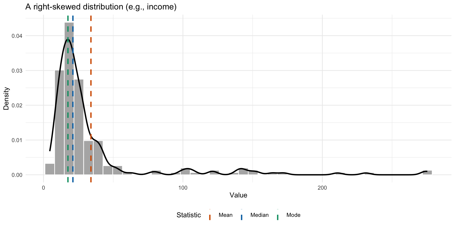
Mean, median, and mode can differ substantially in skewed distributions
When are they the same?
- When the distribution is symmetric and unimodal
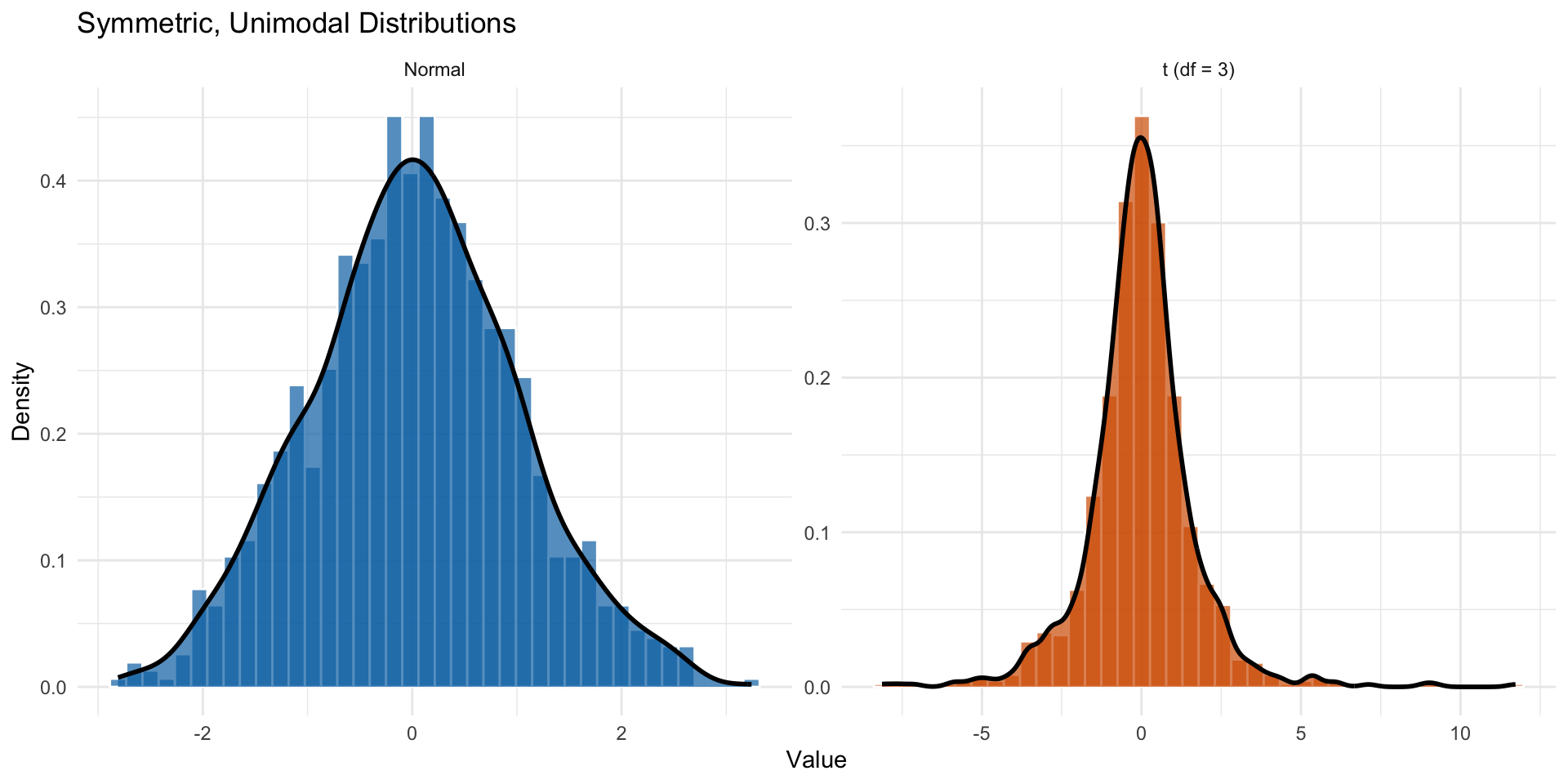
Two symmetric and unimodal distributions: Normal and t-distribution
Comparing the measures
| Feature | Mode | Median | Mean |
|---|---|---|---|
| Intuition | Most typical | The middle | Balance point |
| Outliers | Ignores them | Ignores them (Robust) | Heavily affected |
| Math use | Difficult | Harder to manipulate | Easiest in formulas |
Why is the mean so dominant?
Lots of contexts (e.g. finance) where the mean is good because it penalizes big errors.
Ease of calculation: Before computers, calculating the median required sorting all the data (very slow for big lists). Calculating the mean just required keeping a running total.
- Also the function minimizing the squared errors is much easier to work with than the function minimizing the absolute errors.
The location and its “errors”
Imagine you must pick one number to predict the next value in a dataset. You will be fined based on how wrong you are.
We call your miss the ‘error’ \(e_i = x_i - g\) where \(x_i\) is the actual value and \(g\) is your guess.
Three different penalty rules lead to three different “best” answers:
- All-or-nothing penalty \(\rightarrow\) Mode
- Linear penalty \(\rightarrow\) Median
- Squared penalty \(\rightarrow\) Mean
The all-or-nothing game
The rule: If you are exactly right, you pay nothing. If you are wrong by any amount, you pay £100.
Best strategy: Pick the Mode. (small caveat: the mode needs to exist)
- It gives you the highest probability of hitting the number exactly.
Loss function: \(L(e) = 100 \times \mathbb{I}(e \neq 0)\)
The linear penalty game
The rule: You pay £1 for every unit you are away from the truth. Being off by 10 costs £10; being off by 100 costs £100.
Best strategy: Pick the Median.
It minimizes the sum of absolute deviations
Balances the distance on the left and right sides
Loss function: \(L(e) = 100 \times |e|\)
The squared penalty game
The rule: You pay based on the square of your error.
- Off by 1? Pay £1.
- Off by 10? Pay £100.
- Off by 50? Pay £2,500.
The logic: Small mistakes are fine, but big mistakes are disastrous.
Best strategy: Pick the Mean.
- It minimizes the sum of squared errors (Least Squares)
Loss function: \(L(e) = 100 \times e^2\)
From location to spread
The problem: Knowing the average isn’t enough.
The average squared error
Recall: The mean is the number that minimizes the sum of squared errors.
The question: If the mean is our “best guess,” how good is that guess on average?
Calculate the squared distance of every point from the mean
Add them up and divide by the count
This gives us a measure of the average dispersion of the data
Variance: definition
Definition: The Variance (\(s^2\)) is the average squared distance from the center.
\[s^2 = \frac{1}{n}\sum_{i=1}^{n}(x_i - \bar{x})^2\]
Translation: “How far, on average, are the data points from the mean (squared)?”
Remember we defined: \(e_i = x_i - \bar{x}\).
So we can rewrite the variance as:
\[s^2 = \frac{1}{n}\sum_{i=1}^{n} e_i^2\]
The units problem
If we measure the age at death of Roman Emperors in years, the variance is measured in years squared
What is a “square year”? It doesn’t make intuitive sense historically.
This is awkward for interpretating variance on the scale of the data
Standard deviation: returning to regular units
The fix: Take the square root of the variance to put the spread in units that are the same as the data.
Definition: The Standard Deviation (\(s\))
\[s = \sqrt{s^2} = \sqrt{\frac{1}{n}\sum_{i=1}^{n} e_i^2}\]
which equals:
\[s = \sqrt{\frac{1}{n}\sum_{i=1}^{n} x_i^2 - \bar{x}^2}\]
Interpretation: Roughly the “average” distance of a data point from the mean.
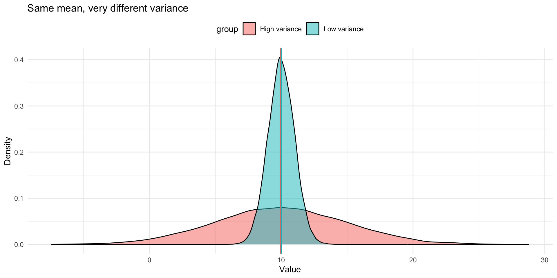
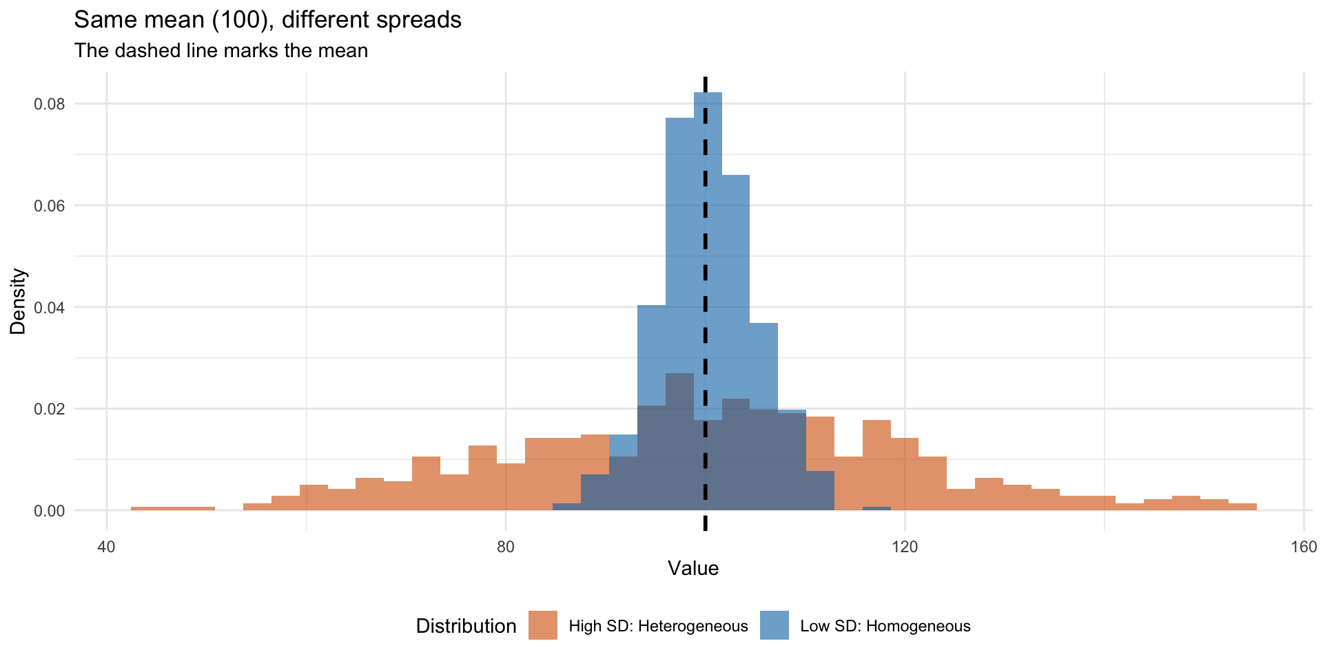
What does the standard deviation tell us?
Low SD: Data is close to the mean
- A more homogeneous population
High SD: Data is far from the mean
- A more heterogeneous population
Two datasets with the same mean but different SDs describe very different worlds
Visualizing dispersion
Other measures of dispersion
Sometimes (not often) you will see other measures of dispersion e.g.
- The range: the difference between the maximum and minimum value
- The interquartile range: the difference between the 75th and 25th percentile
- The mean absolute deviation: the average absolute distance from the mean
- The median absolute deviation: the median of the absolute distances from the median
Means and sample averages
Imagine a well defined population like “the heights (in cm) of all students currently registered in the history department at KCL”
- Imagine this is 1000 students
This population has a mean which we will call \(\mu\) (it is convention to use the greek letter mu for the population mean)
This population has a standard deviation which we will call \(\sigma\) (it is convention to use the greek letter sigma for the population standard deviation)
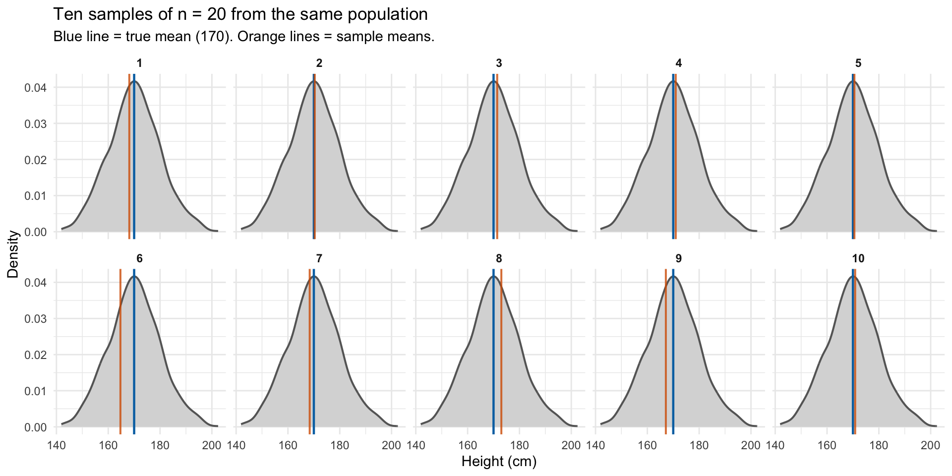
I take the heights of the ~20 history students in this class and calculate the average height \(\bar{x}\)
What is the relationship between \(\bar{x}\) and \(\mu\)?
Means and sample averages
Sample vs population
In practice we rarely observe the full population
We observe a sample and want to learn about the population
Sample statistics are estimates of population parameters
| Population parameter | Sample statistic |
|---|---|
| \(\mu\) (mean) | \(\bar{x}\) |
| \(\sigma^2\) (variance) | \(s^2\) |
| \(\sigma\) (std dev) | \(s\) |
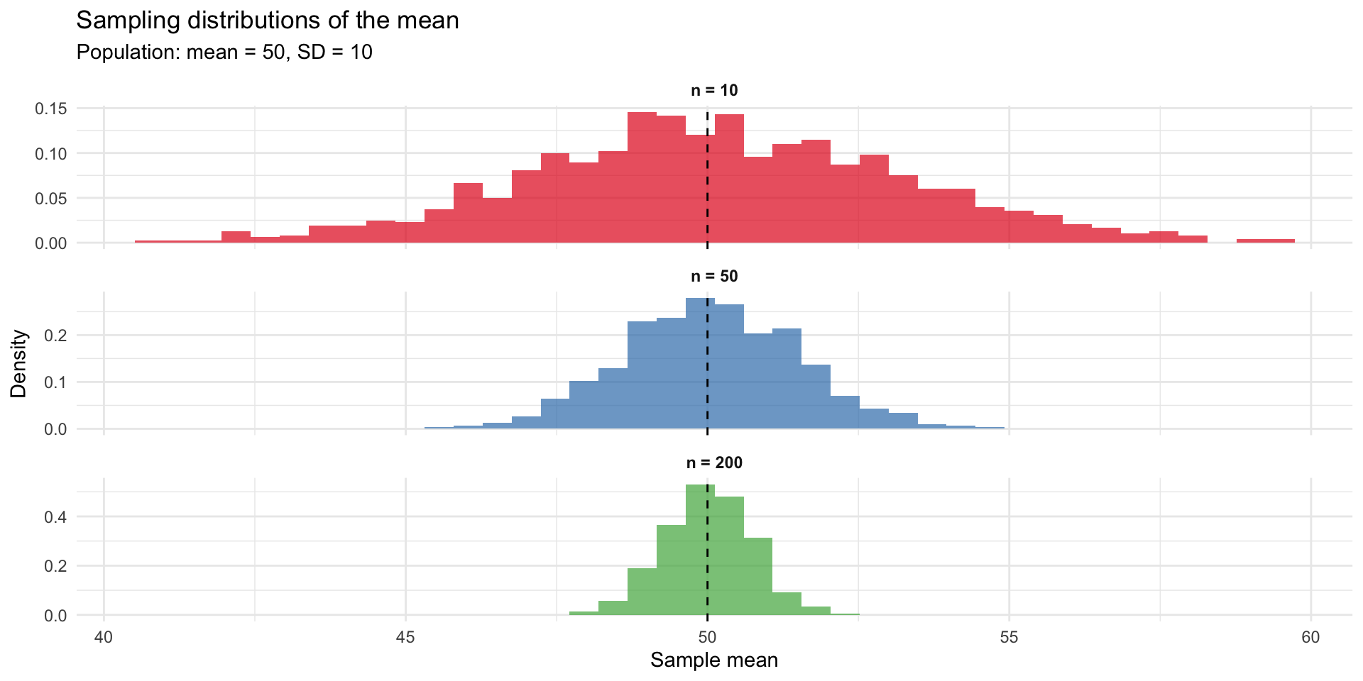
The sampling distribution
A sample mean is itself subject to sampling error
If we drew many samples from the same population, each would give a different \(\bar{x}\)
The distribution of these sample means is called the sampling distribution
This distribution has its own spread, which we can quantify
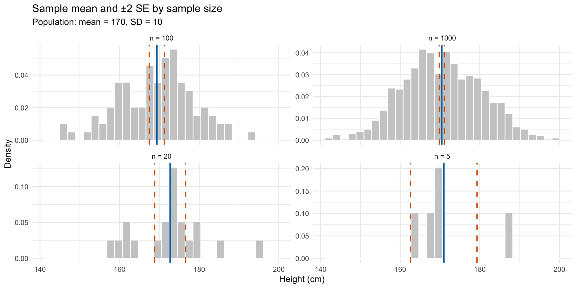
The standard error of the mean
The standard error of the mean (SEM) describes how much sample means vary:
\[SE(\bar{x}) = \frac{\sigma}{\sqrt{n}}\]
Key insight: the standard error decreases as sample size increases
Larger samples give more precise estimates
The standard error and sample size
Standard deviation vs standard error
| Standard Deviation (SD) | Standard Error (SE) | |
|---|---|---|
| Measures | Spread of individual observations | Spread of sample means |
| Question | How variable is the data? | How uncertain is our estimate of the mean? |
| Formula | \(s = \sqrt{\frac{1}{n}\sum(x_i - \bar{x})^2}\) | \(SE = \frac{s}{\sqrt{n}}\) |
| As n increases | Stays roughly the same | Gets smaller |
| Describes | The population/sample itself | Our knowledge about the population |
Intuition for the standard error
Why the standard error matters
The standard error lets us quantify uncertainty about our estimate
Larger samples give more precise estimates (smaller SE)
This is the foundation for:
- Confidence intervals
- Hypothesis testing
- Assessing statistical significance
Statistical vs substantive significance
The standard error is what is used to determine if something is ‘statistically significantly different’ from another thing (usually zero)
That is because confidence intervals are constructed using the standard error (we discussed CIs last week)
The bigger your sample the smaller the CI
McCloskey and Ziliak (1996) insists we should not confuse statistical significance with substantive significance
Statistical significance is about how precisely we measure something, not how big something is.
Key takeaways
Location (mean, median, mode) tells us where the center is – each minimizes a different type of error
Scale (variance, standard deviation) tells us how spread out the data is
The standard error tells us how uncertain we are about our estimate of the mean (it is the standard deviation of our parameter of interest)
Bibliography
McCloskey, Deirdre N., and Stephen T. Ziliak. 1996. “The Standard Error of Regressions.” Journal of Economic Literature 34 (1): 97–114. http://www.jstor.org/stable/2729411.
Stigler, Stephen M. 2016. The seven pillars of statistical wisdom. Cambridge, Massachusetts London, England: Harvard University Press.