
Measurement Error
Gabriel Mesevage
Today’s plan
- Classical measurement error and why averaging works
- Systematic but uncorrelated bias: we can still recover \(\beta\)
- Non-classical (correlated) bias: destroys inference
- Measurement error in the explanatory variable: attenuation bias
- Application: population data, Nunn & Qian, and Guinnane’s critique
What is classical measurement error?
Any measurement of a true quantity \(\tau^*\) will contain some error
We write the measured value as \(\tau_i = \tau^* + \epsilon_i\)
Classical measurement error has three properties:
- Mean-zero: errors are symmetric — as often too high as too low, \(E[\epsilon_i] = 0\)
- Uncorrelated with the true value: big things are not measured with bigger errors
- Uncorrelated with other errors: e.g. in a regression
Under these conditions, averaging works:
\[\text{Avg}(\tau_i) = \frac{1}{N}\sum_i \tau_i = \tau^* + \underbrace{\text{Avg}(\epsilon_i)}_{\to\, 0} \xrightarrow{N \to \infty} \tau^*\]
- Key result: with enough measurements, the errors cancel and we recover the truth
The experiment — round 1
I will toss a book in the air. Time how long it stays in the air (seconds, to 2 decimal places) and enter your measurement in the spreadsheet.
What is systematic bias?
Classical measurement error assumes errors are mean-zero — but what if they are not?
Systematic bias: the average error is not zero, \(E[\epsilon_i] = b \neq 0\)
Example: when timing the book-toss, students may be systematically slow to hit stop — over-estimating time in the air on average
This is a constant bias — it shifts every measurement by the same amount
The good news: if the bias does not depend on what you are measuring, it can still be harmless for many purposes
Specifically, if the bias is the same across all groups being compared, it cancels in the comparison — as we will now show
Systematic bias in the experiment
- Let \(D_i = 1\) if the toss is right-handed, \(D_i = 0\) if left-handed
- Suppose the bias \(b\) is the same whichever hand I use:
\[\tau_i = D_i \tau^R + (1-D_i)\tau^L + b + \epsilon_i\]
Rearranging step by step:
\[\tau_i = D_i \tau^R + \tau^L - D_i \tau^L + b + \epsilon_i\]
\[\tau_i = \underbrace{\tau^L + b}_{\alpha} + \underbrace{(\tau^R - \tau^L)}_{\beta}\, D_i + \epsilon_i\]
The regression coefficient \(\beta\) still estimates the true difference between right and left-handed tosses
The bias is absorbed entirely into the intercept \(\alpha\)
Intuition: if you make the same mistake measuring both groups, the mistake cancels when you take the difference
The experiment — round 2
The data from round 1 (right-hand toss) is still in the spreadsheet. Now open the sheet and add a left-hand toss only — record the time and mark which hand.

Non-classical bias: the algebra
- Now suppose the bias is different for the two groups: \(b^R\) for right-hand, \(b^L\) for left-hand
- The bias is correlated with the treatment \(D_i\)
Starting from:
\[\tau_i = D_i(\tau^R + b^R) + (1-D_i)(\tau^L + b^L) + \epsilon_i\]
Expanding:
\[\tau_i = D_i(\tau^R + b^R) + (\tau^L + b^L) - D_i(\tau^L + b^L) + \epsilon_i\]
\[\tau_i = \underbrace{(\tau^L + b^L)}_{\alpha} + \underbrace{[(\tau^R - \tau^L) + (b^R - b^L)]}_{\beta}\, D_i + \epsilon_i\]
- The slope \(\beta\) now mixes together the true difference \((\tau^R - \tau^L)\) and the bias difference \((b^R - b^L)\)
Non-classical bias: what it means
We cannot separate the true difference from the bias difference — they are bundled into a single number \(\hat\beta\)
A finding of \(\hat\beta = 1\) second is consistent with any of:
- A real 1-second gap, zero bias difference
- No real gap, a 1-second bias difference
- A 2-second real gap offset by a −1-second bias difference
- … and infinitely many other combinations
Sometimes context or logic lets us put reasonable bounds on the biases — but not in general
Lesson: measurement error that is correlated with your explanatory variable destroys inference — you cannot recover the true relationship
Measurement error in the explanatory variable
So far the error has been in the outcome \(\tau_i\). What if the error is in the explanatory variable?
True model: \(y_i = \alpha + \beta x^*_i + \epsilon_i\), but we observe \(x_i = x^*_i + u_i\)
Assume classical \(u_i\): mean-zero, uncorrelated with \(x^*_i\) and \(\epsilon_i\)
Recall \(\hat\beta = \text{Cov}(x_i, y_i) / \text{Var}(x_i)\). Substituting:
\[\text{Cov}(x_i, y_i) = \text{Cov}(x^*_i + u_i,\; \beta x^*_i + \epsilon_i) = \beta\,\text{Var}(x^*_i)\]
\[\text{Var}(x_i) = \text{Var}(x^*_i) + \text{Var}(u_i)\]
Therefore:
\[\hat\beta = \beta \cdot \frac{\text{Var}(x^*_i)}{\text{Var}(x^*_i) + \text{Var}(u_i)}\]
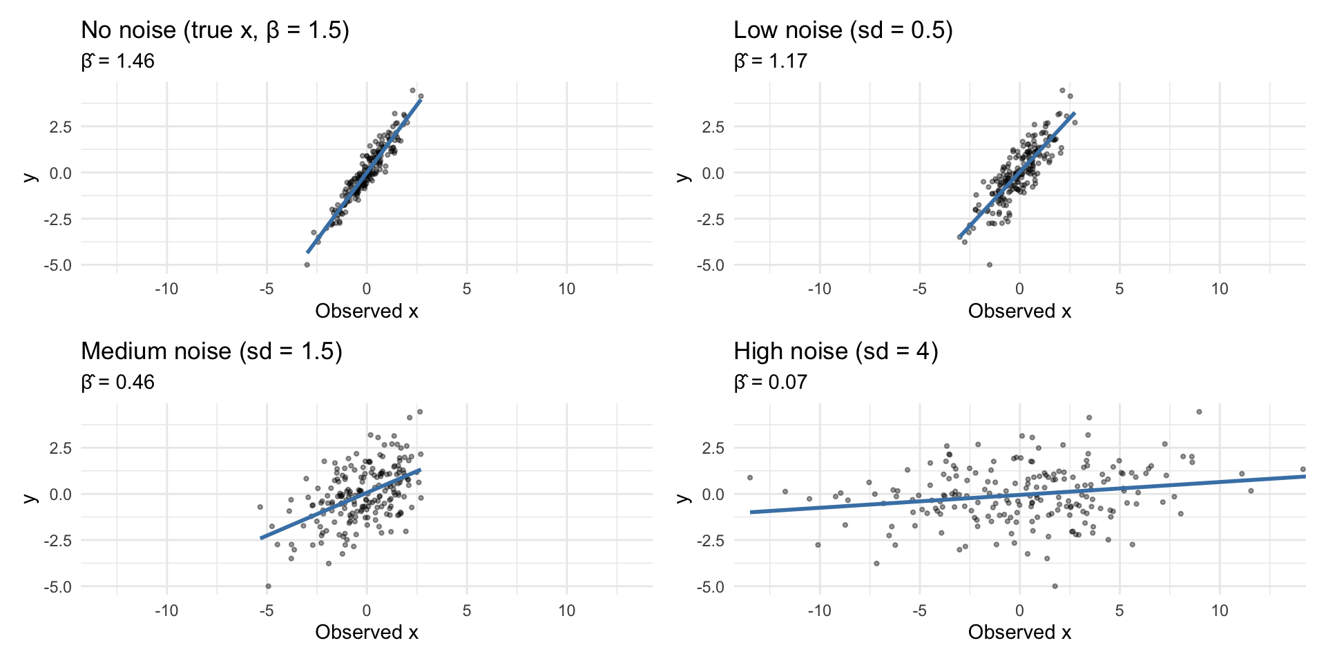
Attenuation bias — implications
\[\hat\beta = \beta \cdot \underbrace{\frac{\text{Var}(x^*_i)}{\text{Var}(x^*_i) + \text{Var}(u_i)}}_{\text{between 0 and 1}}\]
The fraction is always between 0 and 1: attenuation bias — \(\hat\beta\) is pushed toward zero
The larger the noise variance \(\text{Var}(u_i)\) relative to the signal, the closer \(\hat\beta\) gets to zero
A constant error (zero variance) causes no bias — it is only variation in the error that attenuates
You will often see scholars argue: “even if there is measurement error, it just makes us under-estimate the relationship” — this is true only for classical error
If error in \(x\) is non-classical, the bias is unknown in sign and magnitude
Moreover: ME in \(x\) corrupts estimates of all other coefficients in a multiple regression, even if their own regressors are perfectly measured
Attenuation bias — visualised
Nunn & Qian: the potato and population
Nunn and Qian (2011) ask: did the introduction of the potato to Europe after 1700 drive population growth?
The potato originated in South America; it spread through Europe unevenly, largely determined by soil and climate suitability
This suitability is plausibly unrelated to other determinants of population growth — which makes it a useful source of variation
Simplified regression:
\[y_{it} = \beta \cdot \text{PotatoSuitable}_i \times \mathbf{1}[\text{After 1700}]_t + \alpha_i + \tau_t + \epsilon_{it}\]
\(y_{it}\): log population; \(\alpha_i\): region fixed effects; \(\tau_t\): period fixed effects
\(\beta\) captures the extra population growth after 1700 in regions more suitable for potatoes
The data: McEvedy & Jones
Population data come from McEvedy & Jones (MJ), Atlas of World Population History
MJ describe their construction process openly. Key features per Guinnane (2023)
- Figures are rounded to the nearest unit (where the unit itself depends on the size of the population)
- Estimates for periods with little evidence rely on perceived level of economic activity
- Growth rates are set to round numbers (e.g. “doubling every century”)
- Countries with thin evidence are benchmarked against neighbours
To use MJ for sub-national regions, researchers allocate population by land area share — a further step not in MJ
Question for discussion: given how this data was constructed, what would you expect the measurement error to look like? Is it likely to be classical?
Bibliography
Guinnane, Timothy W. 2023. “We Do Not Know the Population of Every Country in the World for the Past Two Thousand Years.” The Journal of Economic History 83 (3): 912–38. https://doi.org/10.1017/S0022050723000293.
Nunn, N., and N. Qian. 2011. “The Potato’s Contribution to Population and Urbanization: Evidence From A Historical Experiment.” The Quarterly Journal of Economics 126 (2): 593–650. https://doi.org/10.1093/qje/qjr009.