| Individual | Height (cm) | Gender | DOB |
|---|---|---|---|
| 1 | 177.4 | M | 1826-10-28 |
| 2 | 167.6 | M | 1829-05-14 |
| 3 | 176.3 | M | 1829-02-20 |
| 1517 | 162.9 | F | 1824-01-18 |
2 Linear Regression
There are different perspectives for motivating regression modelling. We are going to focus on a simple understanding of regression as a way of comparing averages (Gelman, Hill, and Vehtari 2020).
2.1 A motivating example
Let’s start with a motivating example: we are back in the world of comparing heights, say for an anthropometric study. I have a dataset of 1,517 heights recorded in 1850. In addition, 1,215 have recorded gender as male and 302 have recorded gender as female. For each record I also measure the person’s date of birth.
I show a snippet of the data below.
2.2 Comparing averages by gender
We are all comfortable with how we would calculate an average here:
\[ \text{Avg} = \sum_{i=1}^{1517} \frac{h_i}{1517} \]
It would be straightforward to calculate these averages separately by gender. The calculations would be
\[ \text{Avg}_M = \sum_{i=1}^{1215} \frac{h_i}{1215} \]
and
\[ \text{Avg}_F = \sum_{i=1}^{302} \frac{h_i}{302} \]
For each of these means we might want to calculate the standard error. As you will recall from earlier lectures, this is the standard deviation divided by the square root of the number of observations.1 Let’s just assume for a minute that the standard deviation of men’s and women’s heights would be the same, and we’ll call this value \(\sigma\). If that’s the case, then the standard error of the male heights is \(\sigma_M = \frac{\sigma}{\sqrt{1215}} \approx \frac{\sigma}{35}\) and the standard error of the female heights is \(\sigma_F = \frac{\sigma}{\sqrt{302}} \approx \frac{\sigma}{17}\). So we can see that our measure of male heights is about \(35/17 \approx 2\) times as accurate as our measure of female heights.
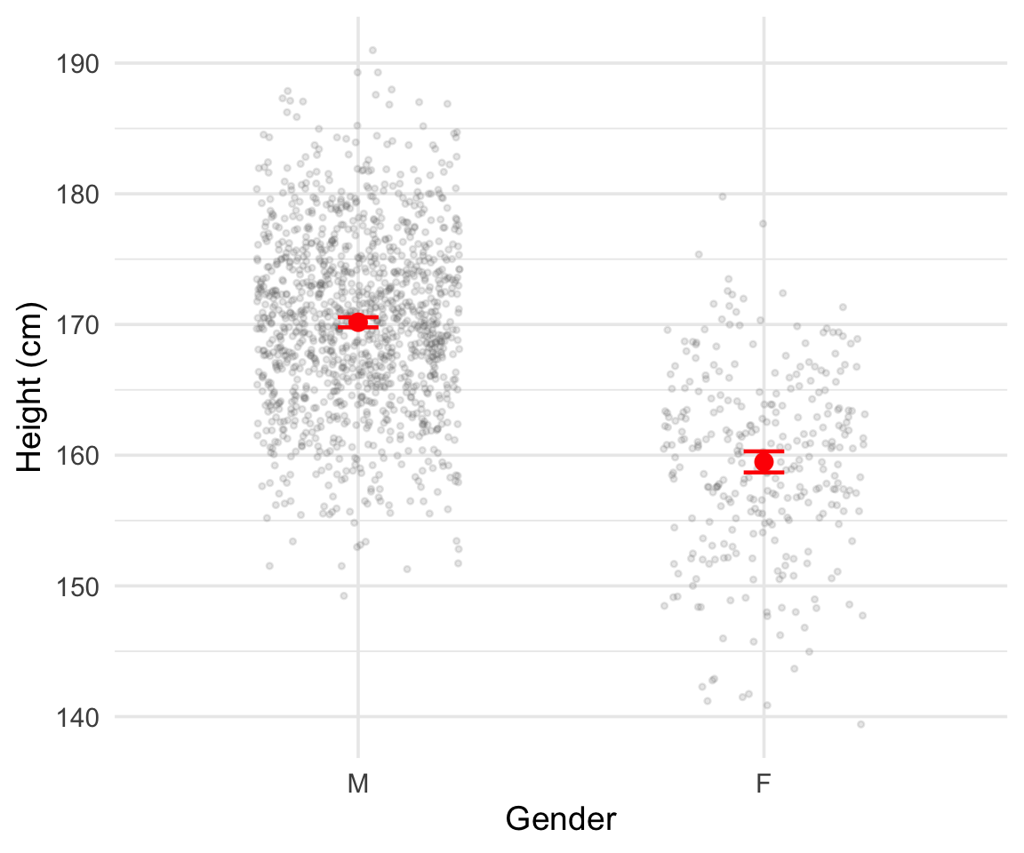
That female heights are measured with less accuracy occurs simply because we observe fewer women in the data. But we still see plenty of female heights so this presents no real difficulty. Below I plot everyone’s heights in two groups, one Male and one Female, and annotate the plot with the calculated average height. I’ve added/subtracted two standard errors from either side of the average.
2.3 Averaging by date of birth
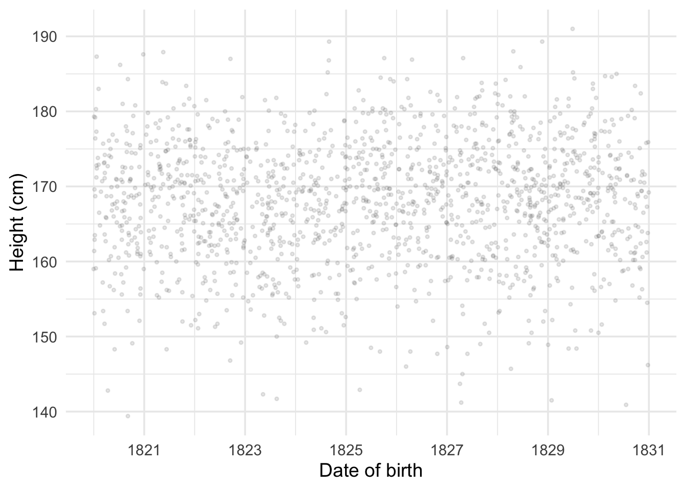
But what if we want to calculate the average by date of birth (DOB)? Let’s start by plotting one against the other.
DOB is measured daily and there are two many different days in our sample to calculate an average for each day. If we reduce date of birth to the year of birth we can in most instances still calculate an average, but it has gotten much less precise. If we work with the year and month of birth it has become almost impossible, and if we work with the actual day of birth most individual days in the year have 1 or no observations. What should we do?
Thinking about prediction. Let’s shift perspective for a minute. Instead of worrying about having enough observations at each date so as to calculate a mean, let’s think about a date we have no observations for and consider a good strategy for guessing what average height would be for the population at this date.
Let’s work the problem looking at the level of year-months. I plot the average of heights by month and year below.
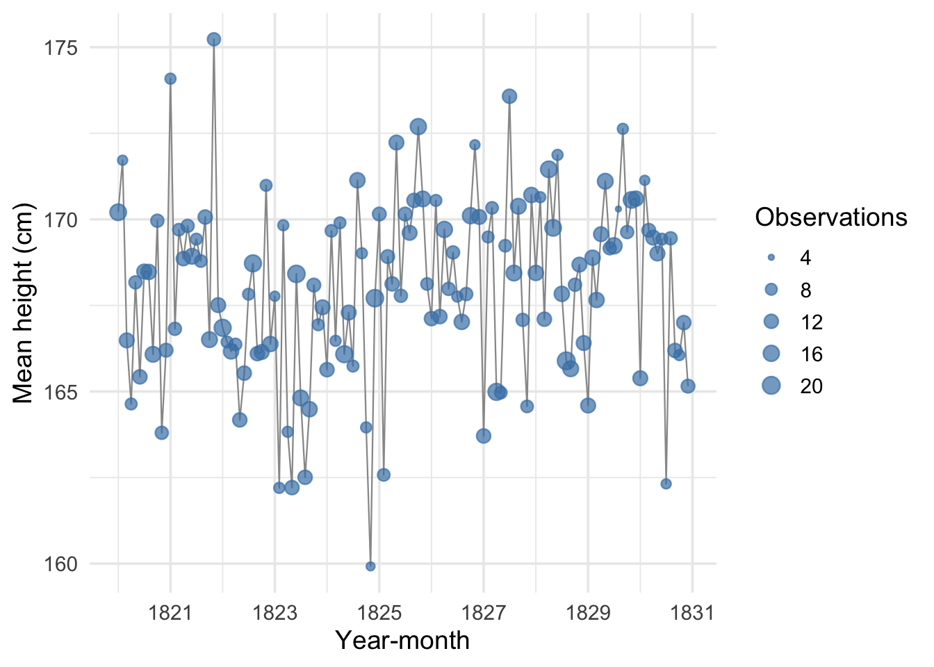
Say we observe a value for average heights in February of 1822, and we observe a value for April of 1822. What would be a reasonable value to infer for March of 1822? One reasonable position might be to say that we don’t know anything about March of 1822 because we have no data and leave it at that. But this seems unreasonably pessimistic. One approach might be to interpolate between the two dates we observe heights for:
\[ \hat{h}_{1822\text{-Mar}} = \frac{h_{1822\text{-Feb}} + h_{1822\text{-Apr}}}{2} \]
Our interpolation is a pretty good approach but has some demerits. First, the individual observations for February and April are not supported by many observations. So they might not be very accurate themselves. In this sense, averaging February and April might make our estimate of average height in March more accurate than our estimates of height in February or April. But that should make us reconsider how we are calculating average height for the people born in April and February, because there is more data available to us that we are not making use of.
Second, we actually observe many year-month data points. Consider the average heights for May 1822. How should we include these? If we had missing heights for two months in a row, say June and July, how would we go about guessing the missing averages?
Finally, we have been working with monthly averages but really we see the day people are born. If someone is born January 31st and another person February 1st, our monthly averages would separate them but really they’re close together in time. We want an approach that 1. uses all of the observed data and 2. generalizes to any date with missing values.
2.4 Conditional averages and linear regression
A good starting point is to clarify what our best case would be: the best case would be so many observations per date that we could simply calculate the average for each day. This would simply be what we call the conditional average: the average conditional on the day a person was born.2
We don’t have that, but at least we know that our goal is a conditional average. What could we do instead? We could try to calculate an average that depends on the date and a very small number of unknown values, which we call parameters.
Linear regression is the solution that computes a linear approximation to that conditional average we are interested in: it is a linear approximation to answering the question “what is average height for people born on a specific date?” The word linear here means (reasonably) that the relationship between DOB and height can be drawn as a straight line. This ‘straight line’ relationship has a few implications. It means:
- The relationship is the same no matter what time period we are looking at: if you move from 1822-02-10 to 1822-02-20 it will have the same effect on the average as moving from 1823-02-10 to 1823-02-20.
- The relationship between the outcome and the predictor — so in our case between height and date of birth — is governed by a single parameter.
2.5 The regression equation
We write the linear regression as
\[ h_i = \alpha + \beta \, d_i + \varepsilon_i \]
Let’s go over the pieces of this equation:
\(h_i\): this is the height outcome that we are measuring. We index the number with a subscript — I am using \(i\) which is conventional — to remind us that this is one out of the 1,517 observations in our data.
\(d_i\): this is the date of birth, expressed in decimal years.3 Once again, I am indexing it with the subscript \(i\) to remind us that this is the \(i\)th observation out of 1,517.
\(\alpha\): this is our first parameter. In a linear regression this is often called the “intercept.” This is because if you plot \(h_i\) against \(d_i\) with height along the y-axis (the vertical axis) the value \(\alpha\) is where our linear regression will “intercept” the y-axis. That is because \(\alpha\) is our prediction for the average value of \(h_i\) when \(d_i = 0\). Since this is a parameter we don’t observe it but need to calculate it (estimate it) from our observed data, just as we do with means and standard deviations.
\(\beta\): this is the parameter that measures the linear association between date of birth and height. Like \(\alpha\) we need to estimate it. The value of \(\beta\) tells us how much the average value of height is predicted to change as your date of birth changes by one year. If I am born in 1822, then a person born one year later would be predicted to be \(\beta\) cm taller than me on average.
\(\varepsilon_i\): this is the Greek letter epsilon and it is the error term. What we are trying to predict is the average height at each date of birth, but not everyone has the average height. The deviation of a person’s height from the average height of someone born on their birthday is the error term.
2.6 Ordinary Least Squares
It’s helpful now to think back to our discussion of the average. We saw in that lecture that the average is the value that minimizes the sum of the squared errors. This approach is exactly how we can construct our estimates of the parameters \(\alpha\) and \(\beta\). That means that what we want to do is solve the problem:
\[ \min_{\alpha,\,\beta} \sum_{i=1}^{1517} \varepsilon_i^2 \]
where in this notation \(min_{\alpha,\,\beta}\) means “find the values of \(\alpha\) and \(\beta\) that minimize the following expression”. The expression we want to minimize is the sum of the squared errors. We can write this out fully as
\[ \varepsilon_i^2 = (h_i - \alpha - \beta \, d_i)^2 \]
We don’t need to worry about how to solve this — suffice to say it is easy to solve on a computer.4 The terms \(\varepsilon_i^2\) are the squared deviations away from our linear approximation to the conditional average. The math is simply saying that we pick the values of \(\alpha\) and \(\beta\) such that we make these squared deviations as small as possible.
2.7 Estimating our first regression
The parameters \(\alpha\) and \(\beta\) define for us a simple straight line that we can use to derive any value of \(h_i\) for any value of \(d_i\). Let’s estimate the regression.
We can plot the fitted regression line over our scatter of individual heights.
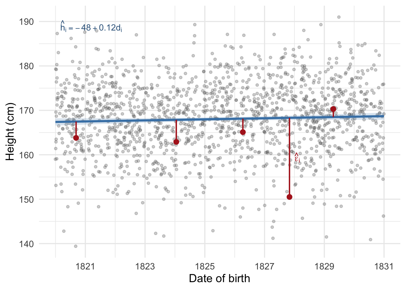
This is a very useful machine! But it should be used with care. Looking at the graph above we can see that the relationship between date of birth and recorded height is slightly positive: the value of \(\hat\beta\) is 0.118 cm per year of birth. What happens if we predict the height using this formula for someone born on 2026-01-01? We would use the linear equation above and the parameters we have estimated. We will follow the convention in statistics and call our estimate of \(\alpha\) “alpha-hat” and write it \(\hat\alpha\), and do the same for \(\beta\) writing our estimate \(\hat\beta\). Our predicted height would be
\[ \hat{h}_{2026\text{-}01\text{-}01} = \hat\alpha + \hat\beta \, d_{2026\text{-}01\text{-}01} \]
which with our data is 191.8 cm. This is absurdly tall for an average height. This absurdity arises because the linear relationship we have found slopes slightly upwards. That upwards rise is true across the dates we are observing, but the machine we have constructed can predict height at any date. Its predictions are likely to be less and less reliable the farther away we move from dates that we actually observe. Moving from dates we actually observe to those we don’t is called predicting off the support of the distribution.
2.8 Errors and residuals
Before we discuss the estimates further, it is important to clarify a distinction that often trips people up: the difference between errors and residuals.
When we wrote down our regression equation, we included the error term \(\varepsilon_i\):
\[ h_i = \alpha + \beta \, d_i + \varepsilon_i \]
This error term is the difference between person \(i\)’s actual height and the true conditional average height for someone born on their date of birth. We never observe this quantity, because we never know the true values of \(\alpha\) and \(\beta\). The error \(\varepsilon_i\) is a theoretical object — it is what we would calculate if we somehow knew the true regression line.
What we do observe are residuals, which we write as \(\hat\varepsilon_i\). These are the differences between the observed heights and the estimated regression line:
\[ \hat\varepsilon_i = h_i - \hat\alpha - \hat\beta \, d_i \]
The hat on \(\hat\varepsilon_i\) reminds us that these are calculated using our estimated parameters \(\hat\alpha\) and \(\hat\beta\), not the true values. The residuals are our best available stand-in for the unknown errors.
Why does this distinction matter? Because when we want to assess the precision of our estimates — how uncertain we are about \(\hat\beta\) — we need to know something about the size of the true errors. We don’t observe them, so we use the residuals as a plug-in estimate. This works well in practice, but it is worth remembering that our measures of uncertainty are themselves estimates, built from the residuals rather than the true errors.
2.9 Statistical uncertainty
Just as with the calculation of a mean, the calculation of the regression coefficients comes from a sample, and is therefore an uncertain measure of the true regression coefficients. Therefore just as with a mean, we need to calculate a standard error that tells us about how precisely our regression coefficients are estimated.
Recall that when we calculate a sample mean \(\bar{h}\), the standard error is
\[ \text{SE}(\bar{h}) = \frac{\hat\sigma}{\sqrt{n}} \]
where \(\hat\sigma\) is the estimated standard deviation of the data and \(n\) is the sample size. We can rewrite this as \(\text{SE}(\bar{h}) = \sqrt{\hat\sigma^2 / n}\). The logic is: we start with how noisy the data are (\(\hat\sigma^2\)), and then we divide by how many observations we have (\(n\)). More noise makes us less certain; more data makes us more certain.
The standard error for a regression slope follows the same logic, but with one important twist. Instead of dividing by the number of observations, we divide by the total spread of the explanatory variable:
\[ \text{SE}(\hat\beta) = \sqrt{\frac{\hat\sigma^2}{\sum_{i=1}^{n}(d_i - \bar{d})^2}} \]
where \(\hat\sigma^2 = \frac{1}{n-2}\sum_{i=1}^{n}\hat\varepsilon_i^2\) is the estimated variance of the residuals (using the residuals \(\hat\varepsilon_i\) as stand-ins for the true errors, as discussed in the previous section).
The numerator plays the same role as before: it measures how noisy the data are around the regression line. But the denominator is different. Why are we dividing by the variance of dates of birth rather than simply the sample size?
The reason is that a regression slope measures a rate of change — cm of height per year of DOB. To pin down a rate of change, what matters is not just how many people we observe but how spread out they are along the x-axis. Imagine two datasets, both with 1,000 observations. In the first, everyone is born within a single month. In the second, births are spread over a decade. Even though both datasets have the same number of observations, the second dataset is far more informative about the slope, because we can see how height changes over a much wider range of dates. The quantity \(\sum(d_i - \bar{d})^2\) captures exactly this: it is larger when dates of birth are more spread out, and this makes \(\text{SE}(\hat\beta)\) smaller.
Notice that \(\sum(d_i - \bar{d})^2\) also grows with \(n\): more observations mechanically increase the total spread. So sample size still helps, just as it does for the mean. But for a regression slope, the distribution of the predictor matters too, not just the count.
2.9.1 Confidence intervals
Using the standard error, we can construct a confidence interval for \(\hat\beta\) just as we did for sample means. The formula is the same as before, but with the standard error of \(\hat\beta\) instead of the standard error of the mean:
\[ \hat\beta \pm ~2 \times \text{SE}(\hat\beta) \]
The correct interpretation of this interval is: if we were to repeat our study many times — drawing a new sample of 1,517 people each time, estimating the regression, and constructing the interval in this way — approximately 95% of those intervals would contain the true value of \(\beta\). Any single interval either contains the truth or it doesn’t, but the procedure of building intervals this way is right 95% of the time.
When zero falls inside the confidence interval, the data are consistent with the possibility that \(\beta = 0\) — that is, no relationship between DOB and height. When zero falls outside the interval, the data suggest the true slope is different from zero. When you see papers in the social sciences discussing ‘statistical significance’ they are typically referring to whether or not the confidence interval includes zero.
2.9.2 The t-statistic
The t-statistic provides a convenient summary of this same information in a single number:
\[ t = \frac{\hat\beta}{\text{SE}(\hat\beta)} \]
This tells us how far away from zero our estimate is, measured in units of standard errors. A useful rule of thumb: when \(|t| > 2\), the coefficient is “statistically significant” at conventional levels, which is equivalent to saying zero lies outside the 95% confidence interval. The bigger the t-statistic in absolute value, the stronger the evidence that the true slope is not zero. You can think of it as measuring the size of the coefficient in units of “how precisely it is estimated” — a coefficient of 0.5 with a standard error of 0.1 (t = 5) is much more convincing than a coefficient of 0.5 with a standard error of 0.4 (t = 1.25).
2.10 Reading a regression table
The estimation of regressions is so common that there has emerged a fairly standard way of presenting the information in a regression in tabular form. Table 2.2 shows the output from our first regression, and it is formatted in a style that you will typically encounter in journal articles.
| Height (cm) | |
|---|---|
| Intercept | −48.229 |
| (118.737) | |
| Date of birth (year) | 0.118+ |
| (0.065) | |
| Num.Obs. | 1517 |
| R2 | 0.002 |
| + p < 0.1, * p < 0.05, ** p < 0.01, *** p < 0.001 |
Let’s walk through the elements of this table:
Coefficient estimates: Each row corresponds to a variable in the regression. The number shown is the point estimate — our best guess for the parameter value. So the row labelled “Date of birth” shows \(\hat\beta\), the estimated change in height (in cm) for a one-year increase in date of birth.
Standard errors in parentheses: Directly below each coefficient is its standard error, enclosed in parentheses. This tells us about the precision of the estimate.
Stars: The stars next to a coefficient indicate its statistical significance. The standard convention is:
+means \(p < 0.1\),*means \(p < 0.05\), and**means \(p < 0.01\). More stars = stronger evidence that the coefficient is different from zero.Intercept: The intercept (\(\hat\alpha\)) is the predicted height when the date of birth variable equals zero. Since our DOB variable is in decimal years, this would be the predicted height for someone “born in year zero”. The intercept is necessary for the regression to work, but we don’t always want to interpret it directly. In our case, the negative value is saying that someone born on the decimal DOB 0000.00 would have a negative height! This is obviously impossible and should remind us of the limitations of extrapolating beyond the range of our data.
R-squared (\(R^2\)): This measures how much of the variation in height is explained by date of birth alone. A value close to 0 means the predictor explains very little of the variation; a value close to 1 means it explains nearly all of it. In our case, \(R^2\) is very low — date of birth alone accounts for very little of the variation in height, which makes sense given the cloud-like scatter we saw in Figure 2.2. It’s common for students to focus on \(R^2\) when first introduced to regression. It has its uses but generally should not be the main focus when interpreting regression results. Its possible for a predictor to explain a very small amount of the variation in the outcome but still have a very large effect. For instance, shark attacks explain a very small amount of the variation in human deaths, but they have a large effect on the probability of death for people who are attacked by sharks. The \(R^2\) is about how much of the variation in the data is explained by the model, which is not always the most interesting question.
Num.Obs. (\(N\)): The number of observations used in the regression.
When I look at a regression table, I tend to focus first on the estimated coefficient and its confidence interval. If the table is reporting standard errors in parentheses, I mentally subtract and add two of them to get a rough 95% confidence interval, and I think about how big that interval is and where it is located (e.g. close to zero or far away from zero). Statistical significance can be interesting but it should not be a point of fixation: the difference between a statistically significant coefficient and a statistically insignificant one can be very small – indeed that difference is likely not statistically significant! It makes sense to look at a confidence interval and a point estimate and ask question like “is this big enough to be substantively meaningful?” and “how precisely is this estimated?” before worrying about the other elements of the table.
2.11 Adding another regressor
We have focused on the relationship between height and DOB, but we have another variable that we know should matter: gender. We can include both predictors simultaneously in a multiple regression. The equation is:
\[ \text{height}_i = \alpha + \beta_1 \cdot \text{dob}_i + \beta_2 \cdot \mathbf{1}[\text{female}_i] + \varepsilon_i \]
where \(\mathbf{1}[\text{female}_i]\) is an indicator variable (sometimes called a “dummy variable”) that equals 1 if person \(i\) is female and 0 if they are male. This is the same minimization problem as before, but now we have three parameters to estimate (\(\alpha\), \(\beta_1\), and \(\beta_2\)) instead of two.
To see what the indicator variable does, consider what the equation predicts for a male versus a female, both born on the same date \(d\):
- For a male (\(\mathbf{1}[\text{female}] = 0\)): the predicted height is \(\alpha + \beta_1 \cdot d + \beta_2 \cdot 0 = \alpha + \beta_1 d\).
- For a female (\(\mathbf{1}[\text{female}] = 1\)): the predicted height is \(\alpha + \beta_1 \cdot d + \beta_2 \cdot 1 = \alpha + \beta_1 d + \beta_2\).
The difference is simply \(\beta_2\). So the coefficient \(\beta_2\) measures the additional increase or decrease to the predicted average height that comes from being in the female group. If women are on average shorter than men, we would expect \(\beta_2\) to be negative. In this way, including a dummy variable for gender is the same as allowing the regression to calculate a separate average level for each group, while still estimating a common slope for DOB.
More generally, multiple regression estimates each coefficient “holding the other variables constant”:
- \(\beta_1\) is the effect of DOB on height holding gender constant — that is, comparing people of the same gender but born at different dates.
- \(\beta_2\) is the average height difference for females relative to males holding DOB constant — that is, comparing men and women born at the same time.
Let’s estimate this model and see what we find.
2.11.1 Visualizing “holding constant”
What does it actually mean to estimate the DOB slope “holding gender constant”? Figure 2.5 walks through the idea step by step in four panels.
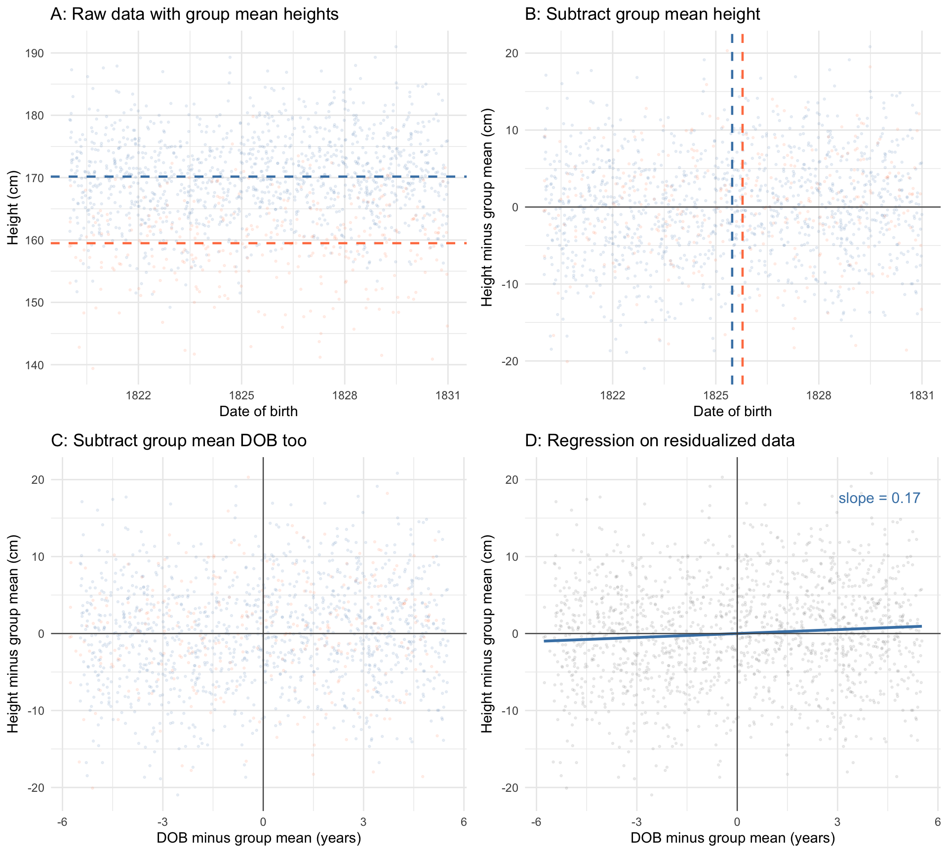
Panel A shows the raw data, coloured by gender, with each group’s average height marked by a dashed horizontal line. The vertical gap between these two lines is the raw average height difference between men and women.
In Panel B, we have subtracted each person’s gender-group average height from their observed height. This removes the level difference between men and women: the two clouds of points now overlap vertically. We have also marked each group’s average date of birth with a dashed vertical line. We can see that these lines are pretty close together, but not the same. This means that on average, women in our sample are born slightly later than men. Our next step is to remove this small different in DOB between the two groups.
In Panel C, we subtracted each person’s gender-group average DOB from their date of birth. Now both variables have been “cleaned” of gender: each individual’s height is now measured as the deviation from their gender’s average height, and each individual’s DOB is measured as the deviation from their gender’s average DOB.
Finally, Panel D fits a regression line through this doubly-residualized data. The slope of this line is exactly \(\hat\beta_1\) from the multiple regression.5 In plain language: the multiple regression coefficient on DOB is what you get when you compare people within their gender group, stripping away the average differences between men and women. Multiple regression is, at its core, about comparing like with like.
2.12 Reading a multiple regression table
Table 2.3 presents both models side by side, which is the conventional way to show how results change as predictors are added.
| (1) | (2) | |
|---|---|---|
| Intercept | −48.229 | −140.962 |
| (118.737) | (100.333) | |
| Date of birth (year) | 0.118* | 0.170*** |
| (0.065) | (0.055) | |
| Female | −10.735*** | |
| (0.434) | ||
| Num.Obs. | 1517 | 1517 |
| R2 | 0.002 | 0.289 |
| R2 Adj. | 0.002 | 0.288 |
| * p < 0.1, ** p < 0.05, *** p < 0.01 |
Several things are worth noting as you compare the two columns:
The DOB coefficient increases between columns (1) and (2). We saw in Figures Figure 2.5 that women were on average shorter, and on average born later. Because of this, the regression line did not rise as steeply as it should have: the rise was muted by the fact that the composition of the sample became less male over time. By adjusting for gender, we isolate how average height is changing over time without the influence of how the gender composition of the sample is changing.
Notice also that the standard error on the DOB coefficient falls substantially in column (2). This is a direct consequence of what we discussed in Section 2.9: the standard error depends on the residual variance \(\hat\sigma^2\). By including gender, we explain a large share of the variation in height, which shrinks the residuals. Smaller residuals mean a smaller \(\hat\sigma^2\), and therefore a more precisely estimated DOB slope. The DOB coefficient gains additional stars in column (2) — not so much because the true effect changed, but because we can now measure it with less noise.
The Female coefficient in column (2) is large and negative, reflecting the well-known average height difference between men and women. As we discussed above, this is the estimated additional shift to average height for being in the female group rather than the male group. The three stars indicate this is statistically significant at the 1% level.
\(R^2\) jumps substantially from column (1) to column (2). Date of birth alone explains very little of the height variation, but adding gender explains a much larger share — because the roughly 10 cm average gap between men and women accounts for a lot of the overall spread in heights.
Adjusted \(R^2\) is a version of \(R^2\) that penalizes for the number of predictors. Because \(R^2\) can only go up (or stay the same) when you add a variable — even a useless one — the adjusted version imposes a small penalty for each additional predictor. When the adjusted \(R^2\) rises meaningfully, as it does here, it is a sign that the added variable genuinely improves the model’s fit.
The same reading conventions apply: coefficients are the main numbers, standard errors sit in parentheses below, stars indicate significance, and the bottom rows show goodness-of-fit statistics. As you read empirical papers in economic history, you will encounter regression tables like this constantly. The ability to quickly parse them — to pick out the coefficient of interest, check its standard error, and assess the overall model fit — is one of the most important skills you can develop.
2.13 Conclusion
Regressions are a work-horse of quantitative social science – and indeed quantitive sciences more broadly. Their ubiquity stems from the fact that they are very simple ways of getting at conditional averages. And the interpretation of regression coefficients is, at its essence, an evaluation of different conditional averages, or how quickly the conditional average changes as the explanatory variable changes.
Regressions are useful but should be evaluated critically. A linear relationship between two variables will slope up or down to infinity as you imagine moving along the x-axis. This is often an absurdity and it is up to the reader to impose sensible limits on where and how the linear regression might apply.
Moreover, as we have seen, the linear regression is a simple linear approximation to the conditional average. That approximation can be quite poor. You should use your background knowledge to evaluate whether you think a linear relationship would be plausible.
Actually you will often see it as dividing by the square root of the number of observations minus 1. This is a “finite sample correction” that arises because we used some of our sample calculating the average. I am going to ignore this distinction for now.↩︎
If you read a statistics or econometrics textbook on this you will often see the object of interest referred to instead as the “conditional expectation”, and see what we have been loosely describing as the ‘average’ described as the ‘expectation’ or ‘expected value’. The word ‘expectation’ is the more mathematically formal way to describe the population average. The ‘expectation’ is the true average for the population, and this helps to clarify when we are talking about calculating an average for a particular collection of data points, and the underlying true average. I have avoided introducing this terminology to keep the exposition simple.↩︎
Dates can be measured as any numerical sequence that walks forwards one unit at a time. A common approach is called the “Unix epoch” and measures time starting at 00:00:00 UTC on January 1, 1970 and counting forwards in seconds (and backwards in negative seconds). We use decimal years so that our coefficient reads as “cm per year of birth.”↩︎
In fact there is a “closed form solution” meaning you could solve it by hand. The solution for \(\beta\) is \(\frac{\text{cov}(d_i, h_i)}{\text{var}(d_i)}\).↩︎
The result that the slope from a regression on residualized data equals the corresponding coefficient from the full multiple regression is known as the Frisch-Waugh-Lovell theorem. It holds exactly, not just approximately, and generalizes to any number of control variables. A formal treatment can be found in most graduate econometrics textbooks.↩︎